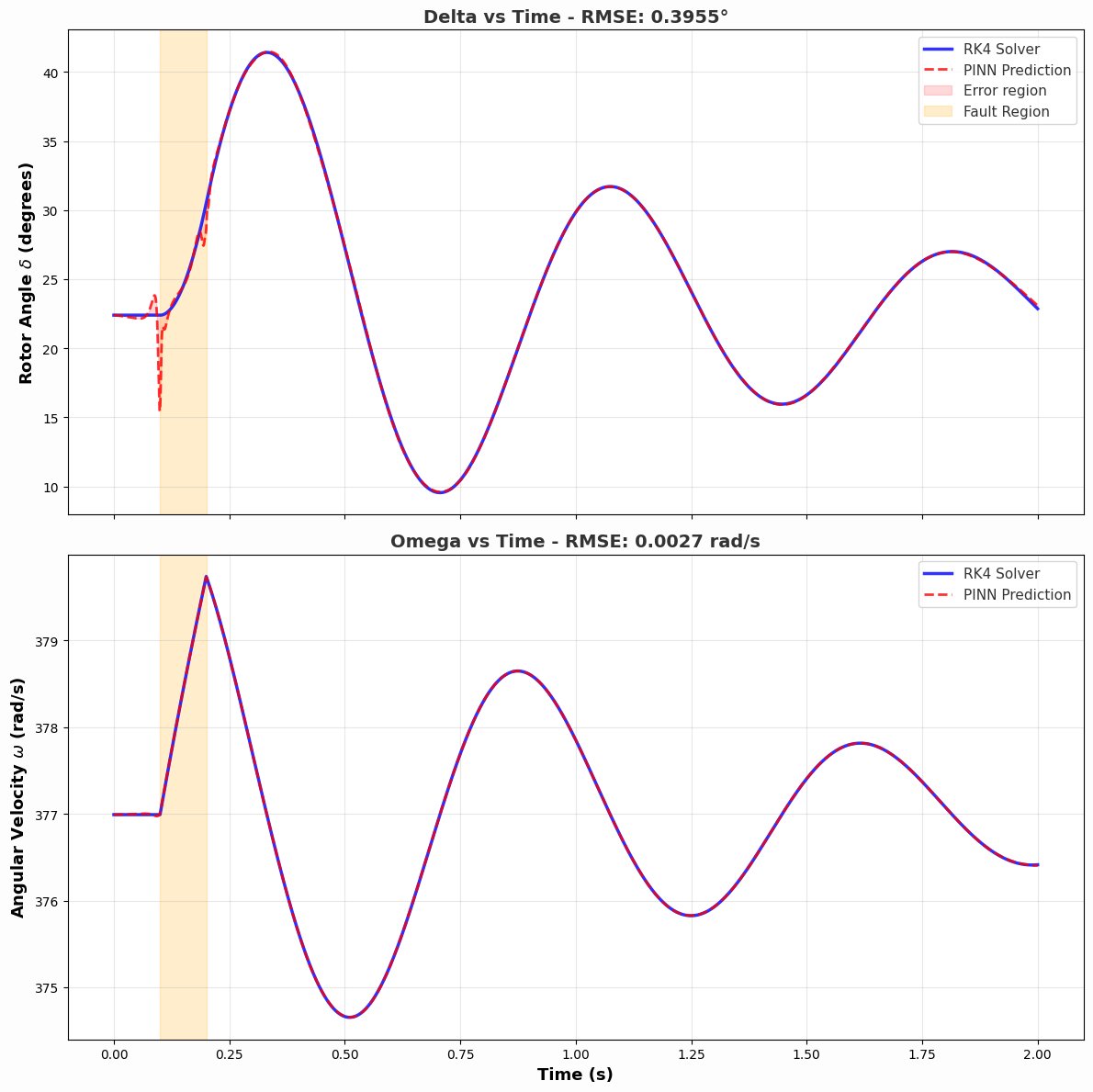
PINN Transient Stability Analysis
Physics-Informed Neural Networks for power system transient stability analysis. Solves the swing equation governing generator rotor dynamics using deep learning with embedded physics constraints, requiring only sparse measurement data.
Overview
Transient stability analysis asks: when a power system experiences a sudden disturbance (fault, line trip, load change), will the generators remain in synchronism or will the system collapse? This project uses a Physics-Informed Neural Network (PINN) to predict rotor angle and angular speed trajectories and map stability boundaries for a Single Machine Infinite Bus (SMIB) system.
Unlike standard neural networks that learn purely from data, the PINN is penalized during training for violating the swing equation. This enforces physical consistency in the predictions and allows accurate results with very few measurement points.
The Physics
The swing equation governs generator rotor dynamics:
2H/ω₀ · d²δ/dt² = Pm - Pe - D·(dδ/dt)
Equivalently as two first-order ODEs:
dδ/dt  = ω - ω₀
dω/dt  = (ω₀ / 2H) · (Pm - Pe - D·ω_dev)
Where δ is rotor angle, ω is angular speed, H is inertia constant, D is damping, Pm is mechanical power, Pe = Pmax·sin(δ) is electrical power output, and ω_dev = ω - ω₀ is speed deviation.
PINN Loss Function
L_total = λ_data · L_data + λ_physics · L_physics + λ_ic · L_ic
The physics residual L_physics is computed using automatic differentiation through the network (torch.autograd.grad), giving exact derivatives without numerical approximation. If the network output satisfies the swing equation, this residual is zero.
Default weights: λ_physics = 1.0, λ_data = 10.0, λ_ic = 100.0
Architecture
| Layer | Size | Activation | Purpose |
|---|---|---|---|
| Input | 1 neuron | Time t (scalar) | |
| Hidden 1-4 | 64 neurons each | Tanh | Learn temporal patterns |
| Output | 2 neurons | Linear | δ(t) and ω(t) |
Tanh is used instead of ReLU because it is infinitely differentiable, enabling clean gradient computation through the network for the physics loss term. Xavier uniform initialization on all linear layers.
System Parameters (SMIB Benchmark)
| Parameter | Symbol | Value | Meaning |
|---|---|---|---|
| Inertia constant | H | 5.0 s | Kinetic energy stored per MVA |
| Damping | D | 0.05 pu | Speed-proportional damping |
| Sync speed | ω₀ | 2π·60 rad/s | Reference angular velocity |
| Mechanical power | Pm | 0.8 pu | Prime mover input |
| Max electrical power | Pmax | 2.1 pu | Peak transferable power |
Training
Two-phase optimization is used, which is standard in the PINN literature:
Phase 1: Adam (5000 epochs, lr=1e-3) — Fast navigation of the loss landscape.
Phase 2: L-BFGS (500 epochs, lr=0.01) — Quasi-Newton fine-tuning for final convergence.
Expected training time: approximately 3 minutes (Adam) + 5 minutes (L-BFGS) on a T4 GPU.
trainer.train_adam(batch, n_epochs=5000, lr=1e-3)
trainer.train_lbfgs(batch, n_epochs=500, lr=0.01)
trainer.save_model('models/pinn_trained.pt')
Results
- RMSE (δ): < 0.5 degrees compared to RK4 reference solution
- RMSE (ω): < 0.01 rad/s
- Critical Clearing Time (CCT): approximately 200 ms for the default SMIB configuration
- 2D stability boundary map over fault duration (50–500 ms) vs initial rotor angle
Outputs
| Plot | Description | Image |
|---|---|---|
rk4_reference.png | Ground truth rotor angle and speed trajectories from RK4 | 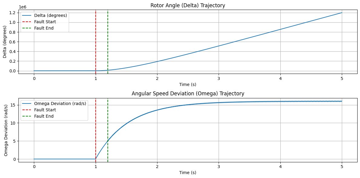 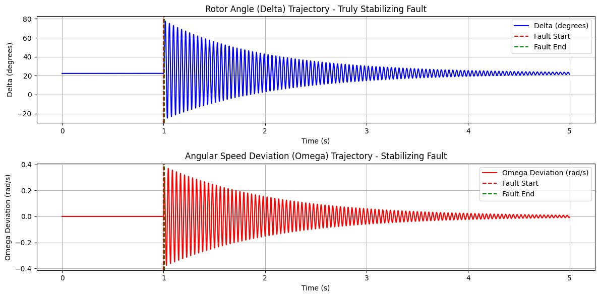 |
training_history.png | Total, physics, and data loss curves on log scale | 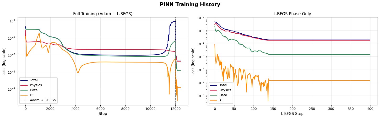 |
pinn_vs_rk4.png | PINN prediction vs RK4 reference with error region | 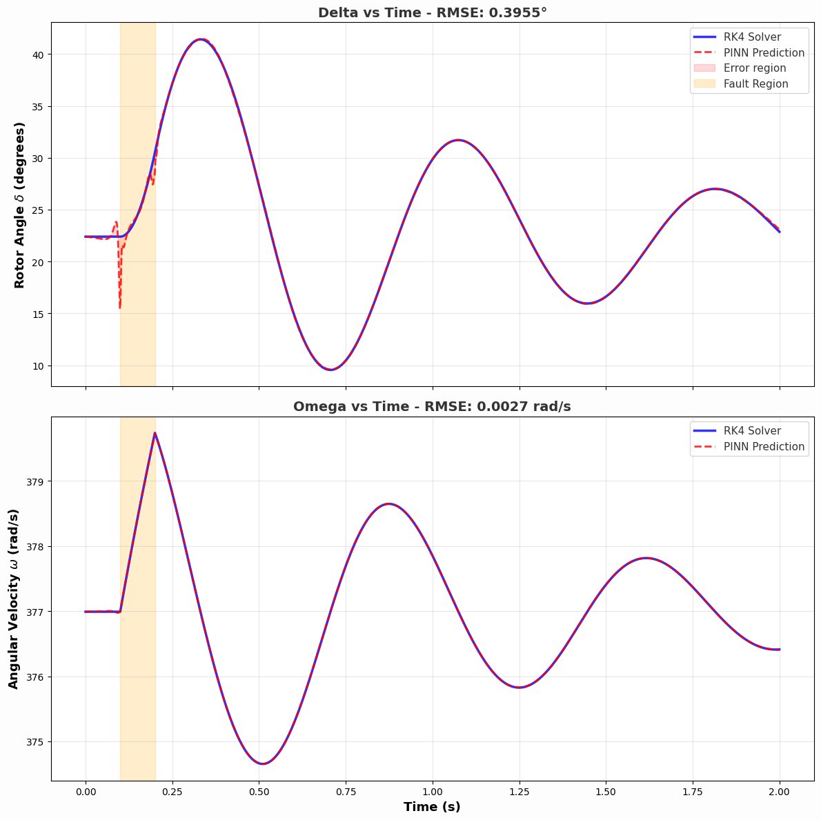 |
stability_boundary.png | 2D stable/unstable classification map | 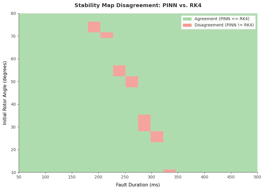 |
phase_portrait.png | δ vs ω phase portrait for multiple fault durations | 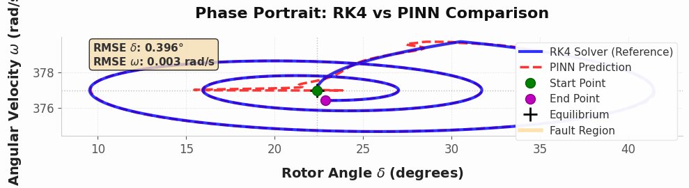 |
Troubleshooting
| Problem | Likely cause | Fix |
|---|---|---|
| Physics loss stays high | λ_physics too low | Increase from 1.0 to 5.0–10.0 |
| Data loss stays high | Too few data points | Increase n_data_points to 100–200 |
| Total loss oscillates | Learning rate too high | Reduce Adam lr to 5e-4 |
| Predictions diverge at t > 1s | Network underfitting | Increase to 6 layers, 128 neurons |
| IC error stays high | λ_ic too low | Increase to 500–1000 |
Dependencies
torch >= 2.0.0
numpy >= 1.24.0
scipy >= 1.10.0
matplotlib >= 3.7.0
scikit-learn >= 1.2.0
tqdm >= 4.65.0
References
- Raissi, Perdikaris & Karniadakis (2019). Physics-informed neural networks. Journal of Computational Physics.
- Misyris, Venzke & Chatzivasileiadis (2020). Physics-Informed Neural Networks for Power Systems. IEEE PES General Meeting.
- Kundur (1994). Power System Stability and Control. McGraw-Hill.