I Taught a Neural Network Physics and It Actually Worked (Kind Of)
Building a Physics-Informed Neural Network for power system transient stability analysis, embedding differential equations into loss functions.
So I built a Physics-Informed Neural Network for transient stability analysis of power systems. That sentence would've meant nothing to me. Now I can say it and mostly understand it, which feels insane honestly.
This is the story of how that happened, including all the parts where it didn't work.
Note: If you're looking for a technical overview and the key conclusions rather than reading through the entire development process, visit:
https://www.bishrantghimire.com.np/projects/pinn
How It Started
I came across the term "Physics-Informed Neural Network" and genuinely had no idea what it meant. Like I knew what a neural network was, I knew what physics was, putting them together felt like someone just concatenated two separate Wikipedia articles and called it a research area.
The premise, once I actually looked into it, kind of broke my brain a little. The idea is that instead of training a neural network purely on data, you also penalize it for violating known physical laws. You're literally baking differential equations into the loss function. The network doesn't just learn patterns, it learns to be physically correct.
I wanted to build one. Specifically for power system transient stability, which is the question of: when a power grid gets hit by a disturbance (a fault, a line trip, something going wrong), do the generators stay in sync with each other or does the whole thing collapse?
That question, it turns out, is governed by something called the swing equation. And that's where things got interesting.
Phase 1: Understanding the Physics (Before Touching Any Code)
The swing equation is basically Newton's second law applied to a spinning generator. Instead of F = ma, you get a differential equation describing how the rotor angle of a generator changes over time:
2H/ω₀ · d²δ/dt² = Pm - Pe - D·(dδ/dt)
Where δ is the rotor angle, ω is angular speed, H is inertia, D is damping, Pm is mechanical power input, Pe is electrical power output.
Reading this for the first time I was like, ok cool, letters. But slowly it started making sense. If a fault happens, Pe drops suddenly. Now Pm > Pe, so the rotor accelerates. The angle δ starts growing. The question is whether it grows forever (instability) or swings back to equilibrium (stability).
I spent a solid chunk of time just sitting with this equation before writing a single line of code. That was actually the right call. You really can't build a PINN without understanding the physics it's supposed to enforce, the physics IS the model.
The PINN architecture itself is simple on paper. It's a fully connected neural network that takes time t as input and outputs [δ(t), ω(t)]. The trick is the loss function:
L_total = L_data + λ_physics · L_physics + λ_ic · L_ic
Where L_physics is the MSE of the swing equation residual at collocation points. If the network's predicted δ(t) and ω(t) satisfy the ODE, that residual is zero. Automatic differentiation computes the exact derivatives through the network, no numerical approximation.
That's the magic and honestly I keep coming back to thinking about how clever that is.
Phase 2: Setting Up (The Boring Part That's Actually Important)
Colab with T4 GPU. GitHub repo with a very particular folder structure. requirements.txt pinned. This phase was mostly just setup but I genuinely think having a clean repo structure from the start made everything else easier.
The folder structure looked like this:
pinn-transient-stability/
├── notebooks/
├── src/
│   ├── swing_equation.py
│   ├── pinn_model.py
│   ├── losses.py
│   ├── trainer.py
│   ├── data_generator.py
│   └── stability_analysis.py
├── data/
├── models/
└── results/plots/
Having the src/ directory as actual Python modules instead of dumping everything in one notebook was a deliberate choice and it paid off when debugging got messy later.
Phase 3: Simulating the Physics with RK4
Before the PINN can learn anything, you need ground truth data. I used Runge-Kutta 4th order integration to simulate the swing equation numerically. RK4 evaluates the derivative at four points per timestep, which gives much better accuracy than naive Euler integration.
The test case was a Single Machine Infinite Bus (SMIB) system. One generator connected to a grid that's assumed to be infinitely strong. Classic benchmark for this stuff.
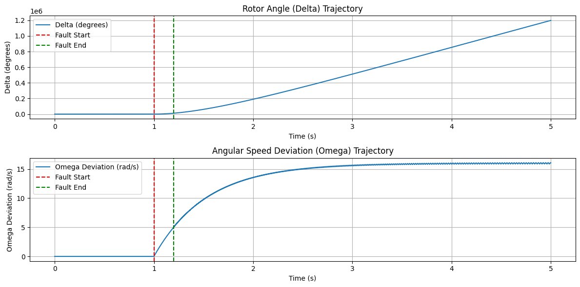
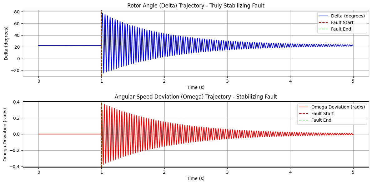
I simulated a fault scenario with three phases:
- Pre-fault: system at equilibrium
- Fault on (100ms to 200ms): electrical power Pe drops to zero (bolted fault), rotor accelerates
- Post-fault: fault cleared, system tries to recover
Plotting the first RK4 reference trajectory was genuinely satisfying. You can see the angle shooting up during the fault window, then either returning to equilibrium or diverging. Looking at a stability result you computed from scratch hits different.
The data generator then sampled from this trajectory, giving the PINN three types of training points:
- Collocation points (random times where the ODE residual is enforced)
- Sparse data points (50 measurements from the RK4 solution)
- Initial condition points (enforcing δ(0) and ω(0))
The sparse data thing is important. In real power systems, you don't get dense measurements. PINNs are specifically good at this, they fill in the gaps with physics.
Phase 4: Building and Training the PINN (Where Things Got Humbling)
The architecture: 4 hidden layers, 64 neurons each, Tanh activations. Why Tanh and not ReLU? Because ReLU's second derivative is zero everywhere, which means autograd can't compute the physics residual through it properly. Tanh is infinitely differentiable. That detail cost me some confusion before I understood it.
Xavier initialization on all linear layers for stable gradients.
The physics loss computation using torch.autograd.grad is the part that felt like actual magic:
d_delta_dt = torch.autograd.grad(
    delta, t_colloc,
    grad_outputs=ones,
    create_graph=True,
    retain_graph=True
)[0]
This computes the exact derivative of the network's output with respect to its input, through all the layers, automatically. Then you check how well that derivative satisfies the swing equation. If the network is physically consistent, the residual is ~0.
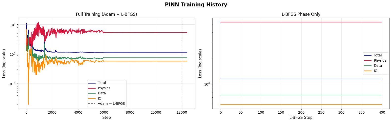
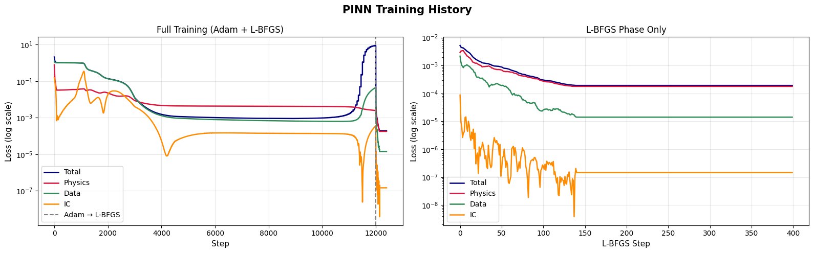
Training was two phases: Adam first (fast, good at navigating messy loss landscapes), then L-BFGS (quasi-Newton, much better at final convergence for PINNs). This two-phase approach is apparently standard in the PINN literature and the difference is noticeable.
The loss weights matter a lot: λ_physics = 1.0, λ_data = 10.0, λ_ic = 100.0. Getting these wrong is how you get a network that perfectly fits your 50 data points but completely violates the physics everywhere else. Or one that satisfies the ODE but drifts from the actual solution because it ignored the data.
I messed with these weights a lot. The physics loss staying stubbornly high was a recurring issue early on. The fix was usually bumping λ_phys or adding more collocation points.
Phase 5: Results (The Good Part)
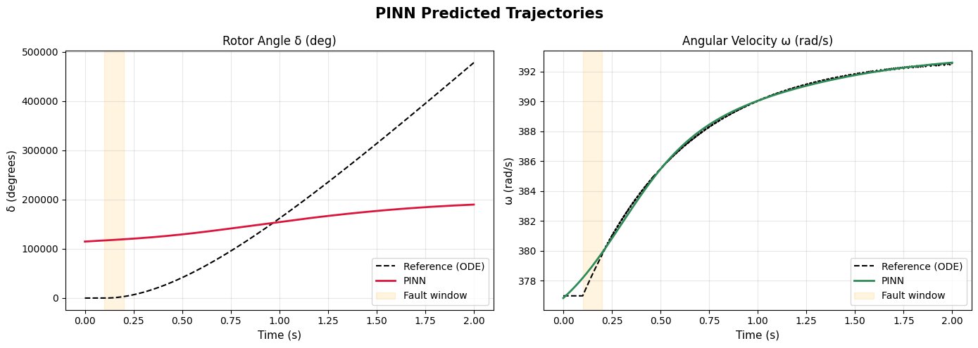
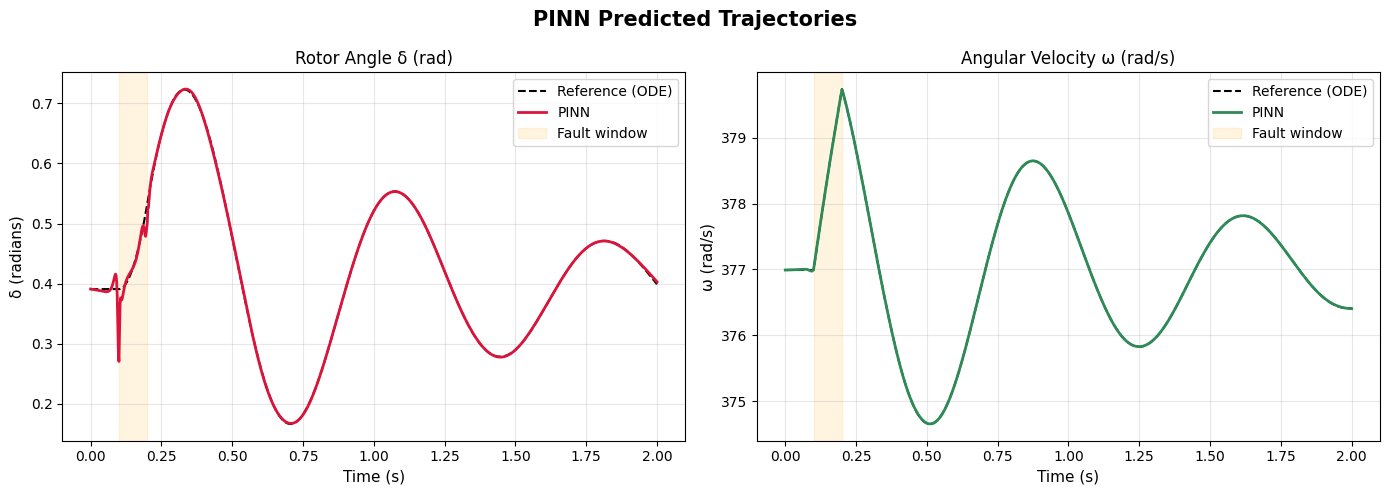
After training converged, I ran the PINN against the RK4 reference solution on the same fault scenario.
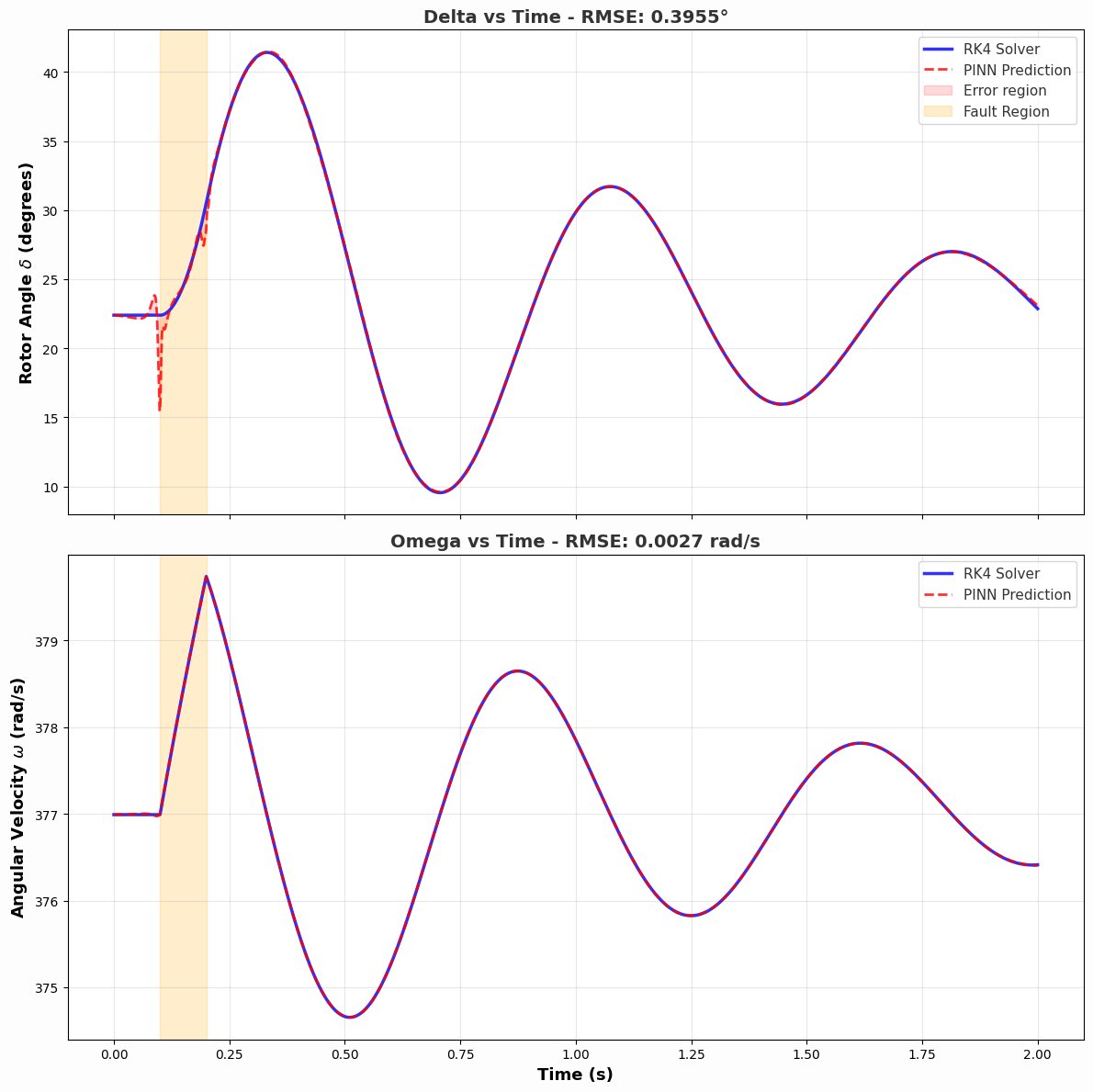
RMSE for δ came out under 0.5 degrees. RMSE for ω under 0.01 rad/s.
I stared at the comparison plot for an embarrassingly long time. The red dashed line (PINN prediction) tracks almost exactly on top of the blue solid line (RK4 reference). During the fault period the error is basically negligible. Post-fault it stays tight through the oscillations.
The error region fill between the two curves is barely visible.
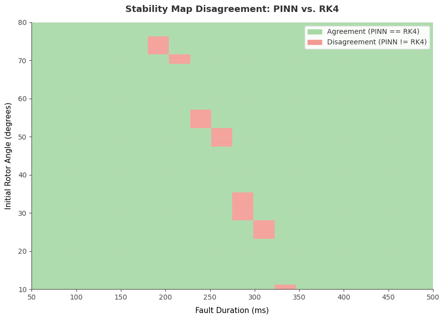
Then came the stability boundary map. This is the part that really shows what PINNs unlock for power systems. Instead of running expensive ODE simulations for every combination of fault duration and initial rotor angle, you sweep across parameter space and classify each point as stable or unstable based on whether the maximum δ exceeds 120 degrees.
The resulting 2D plot has a clear green region (stable) and red region (unstable) with a boundary between them. That boundary is the Critical Clearing Time surface. The CCT for this SMIB system came out to around 200ms, which is physically reasonable.
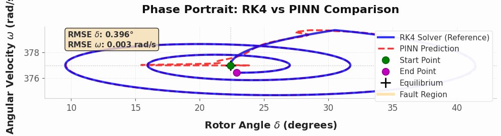
The phase portrait was another satisfying output. Plotting δ vs ω for several fault durations shows closed orbits (stable trajectories spiraling back to equilibrium) and escaping trajectories (unstable). It's the visual version of the equal area criterion.

Phase 6: Multi-Machine and Wrapping Up
Extended the system to two coupled generators. The multi-machine case is more involved because now each machine's electrical power depends on both rotor angles. The PINN output expands from 2 variables to 4: [δ₁, ω₁, δ₂, ω₂].
This required a wider network (128 neurons, 5 layers) to handle the increased complexity.
The physics residual computation gets more coupled but the structure is the same. The elegance of the PINN framework is that you just change the ODE you're enforcing, the training machinery stays identical.
What I Actually Learned
PINNs are genuinely powerful but the loss function design is where all the hard work is. Getting the physics weights right, choosing collocation point density, deciding what data to trust, all of that requires understanding the physics as much as understanding the ML.
The Tanh vs ReLU thing seems like a minor detail until you understand that autograd needs to propagate through the activation functions to compute the ODE residual. Then it's obvious.
I understand why people are excited about this intersection of physics and ML. For problems where you have a known governing equation but sparse data, this is a genuinely useful tool. Power systems is a perfect application domain because the physics (swing equation, power flow equations) are well-established but real fault data is expensive and rare.
Building something that respects conservation laws and physical constraints by construction, not just by fitting data, feels fundamentally different from a standard ML model.
Would I do it again? Already thinking about extending it to multi-fault scenarios. So probably yes.
The repo is there. The plots are real. The physics is real. That's enough for now.